This is paper is available on arxiv under CC 4.0 DEED license.
Authors:
(1) Leah Chrestien, Czech Technical University in Prague;
(2) Tomá˘s Pevný, Czech Technical University in Prague, and Gen Digital, Inc.;
(3) Stefan Edelkamp, Czech Technical University in Prague;
(4) Antonín Komenda, Czech Technical University in Prague.
Table of Links
- Abstract & Introduction
- Preliminaries
- Conditions on strictly optimally efficient heuristic
- Loss functions
- Related Work
- Experiments
- Conclusion and References
- Appendix
8 Appendix
8.1 Speed of convergence against the size of training set:
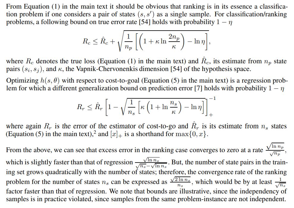
We use the classical results of statistical learning theory to show that estimating the cost-to-go converges more slowly with respect to the size of the training set than estimating the rank.
8.2 Suboptimality of perfect heuristic in GBFS
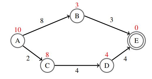
Example 2. While cost-to-goal h∗ is the best possible heuristic for algorithms like A* (up to tiebreaking) in terms of nodes being expanded, for GBFS, h∗ does not necessarily yield optimal solutions.
Proof. A* explores all the nodes with f(s) < f ∗ (s) = g(s)+h∗ (s) and some with f(s) = f∗ (s) = g(s) + h∗ (s), so nodes can only be saved with optimal f∗ (s) = g(s) + h∗ (s). In fact, when given h∗ as the heuristic, only nodes s with f(s) = f∗ (s) are expanded. Depending on the strategy of tie-breaking, the solution path can be found in the minimal number of node expansions or take significantly longer (e.g., in lower g-value first exploration of the search frontier). Any heuristic other than h∗ is either overestimating, and, therefore, may lead to either non-optimal solutions in A*, or weaker than h∗, leading to more nodes being expanded.
Even if h∗ is given, GBFS is not guaranteed to be optimal. Consider the following graph with five nodes A, B, C, D, E, and w(A, B) = 8, w(B, E) = 3, w(A, C) = 2, w(C, D) = 4, w(D, E) = 4, and h ∗ (A) = 10, h∗ (B) = 3, h∗ (C) = 8, h∗ (D) = 4, h∗ (E) = 0 (see Figure 2), initial node s0 = A, goal node E ∈ S∗. The numbers are the actual costs and the red numbers are the exact heuristic function. For finding a path from node A to node E, GBFS would return (A, B, E) following the heuristic function. However, the path (A, C, D, E) has cost 10 instead of 11.
8.3 Theory
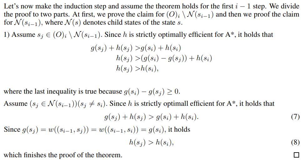
Below, we prove the claim in made in Experimental section stating that if a heuristic h is strictly optimally efficient for A* search, then it is also strictly optimally efficient for GBFS.

We carry the proof by induction with respect to the number of expanded states.
At the initialization (step 0) the claim trivially holds as the Open list contains just a root node and the set of inequalities is empty.
8.4 Optimally efficient heuristic might not exists for GBFS
Consider the following graph in Figure 3 with four nodes A, B, C, D,, and w(A, B) = 1, w(B, D) = 1, w(A, C) = 1, w(A, D) = 9, w(B, C) = 9, and h∗ (A) = 0, h∗ (B) = 1, h∗ (C) = 1, h∗ (D) = 2 where A is the goal state and D is the initial state.
We can see that for GBFS, the perfect heuristic does not exist for D. On expansion, the GBFS algorithm will put A and B to the open list with heuristic values h(A) = 0 and h(B) = 1. GBFS takes A from the open list and checks if it is a goal state. Since A is goal state, GBFS terminates returning path (D,A) as a solution. However, this is not the optimal path as a better (optimal) solution exists (D, B, A). Since the definition of optimal ranking requires the inequalities to hold for this optimal path, in GBFS, the perfect heuristic does not exist for all initial states.
The problem can be fixed if the definition of optimal ranking is changed to consider two cases in the merit function f(s) = αg(s) + βh(s): α > 0 and β > 0 and α = 0 and β > 0 . In the first case, the optimal ranking should be defined with respect to the "optimal path" (this is the A*); in the latter case, it should be the path with minimal number of expansions. With GBFS, the user simply wants to find a solution but not care about its optimality. With this change, the heuristic function will exist for Figure 3.
8.5 Training set with multiple solution paths with the same length of the plan
The behavior of the learned heuristic function depends on the composition of the training set, which is illustrated below on a simple grid problem. The agent starts at position (4,4) and has to move to the goal position (0,0). There are no obstacles and the agent can only move one tile down or one tile left (the effects on his positions are either (-1,0) or (0,-1)), the cost of the action is one. The number of different solutions path grows exponentially with the size of the grid and all solution path has the same cost (for problem of size 5x5, there are 70 solutions). This problem is interesting, since merit function in A* with optimal heuristic function (cost to goal) is constant, equal to 8, for all states.
For the size of the grid (4,4), the heuristic is determined by a table with 25 values. Below, these
values are determined by minimizing the proposed loss for A* algorithm with logistic loss surrogate by BFGS (with all zeros as initial solution). Since the loss function is convex, BFGS finds the solution quickly.
In the first case, the training set contains one solution path ([4, 4], [3, 4], [2, 4], [1, 4], [0, 4], [0, 3],
[0, 2], [0, 1], [0, 0]), where the agent first goes left and then down. The learnt heuristic values h is
shown in Table 2.
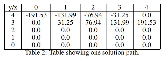
An A* search using these heuristic values will first always take action moving the agent to left and then down. When moving down, the agent does not have another choice. Notice that the heuristic values of many states are not affected by the optimization, because they are not needed to effectively solve the problem.
In the second case, the training set contains two solution paths: the first is in Table 2 and in the second table 3, the agent goes first down and then left. The learnt heuristic values are shown in 3.
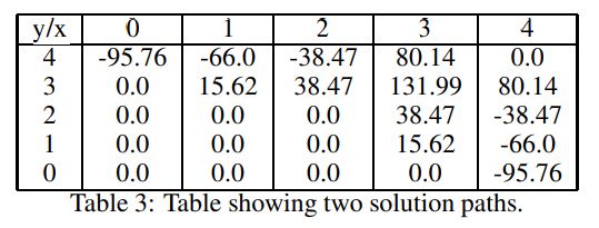
An A* search will now face tie at state (4,4), since states (3,4) and (4,3) have the same heuristic value. But the presence of the tie does not affect the optimal efficiency of the search, as A* will always expand states on one of the optimal path from the training set.
Finally let’s consider a case, where all 70 possible solutions are in the training set. The learned heuristic values are shown in Table 4.
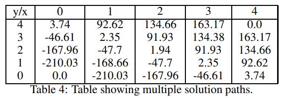
Rank of heuristic values "roughly" corresponds to cost to goal. The reason, why some states are preferred over the others despite their true cost-to-goal being the same is that they appear in more solution paths. As shown in Table 4, the A* search with learnt heuristic values is strictly optimally efficient.
8.6 Baseline Comparison to breadth-first search
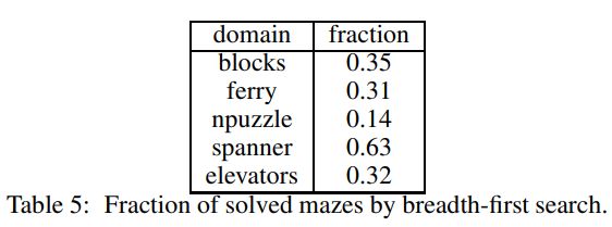
The fraction of solved problems for breadth-first search (5stime limit as used by solvers in the paper) is shown in Table 5.
8.7 Training Details
For the grid domains, ADAM [26] training algorithm was run for 100 × 20000 steps for the grid domains.The experiments were conducted in the Keras-2.4.3 framework with Tensorflow-2.3.1 as the backend. While all solvers were always executed on the CPU, the training used an NVIDIA Tesla GPU model V100-SXM2-32GB. Forward search algorithms were given 10 mins to solve each problem instance.
For the PDDL domains, the training consumed approximately 100 GPU hours and evaluation consumed 1000 CPU hours.All training and evaluation were done on single-core Intel Xeon Silver 4110 CPU 2.10GHz with a memory limit of 128GB. The training algorithm AdaBelief [63] was allowed to do 10000 steps on the CPU. We emphasize though, that the training time does not include the cost of creating the training set.
