Authors:
(1) Jo˜ao Almeida, CEGIST, Instituto Superior T´ecnico, Universidade de Lisboa Portugal;
(2) Jos´e Rui Figueira, CEGIST, Instituto Superior T´ecnico, Universidade de Lisboa Portugal;
(3) Alexandre P. Francisco, INESC-ID, Instituto Superior T´ecnico, Universidade de Lisboa Portugal;
(4) Daniel Santos, CEGIST, Instituto Superior T´ecnico, Universidade de Lisboa Portugal.
5 Computational experiments
In this section, we address the computational experiments. In Subsection 5.1, we test several stopping criteria parameters for smaller instances. In Subsection 5.2, we present the results of instance decomposition with fixed curriculum increments for smaller instances. In Subsection 5.3, we present the results of instance decomposition with violations based curriculum increments for smaller instances. In Subsection 5.4, we test the meta-heuristic with larger subdivisions and the real-world instance. In Subsection 5.5, we present the experiments with the adapted ITC 2007 CBCT instances.
All algorithms are implemented in C++. For the IST instances, the CPU is an 11th Gen Intel(R) Core(TM) i5-11400 @ 2.60GHz 2.59 GHz, and the installed RAM is 16.0 GB (15.8 GB usable). For the adapted competition instances, the CPU is an Intel(R) Core(TM) i7-8565U CPU @ 1.80GHz 1.99 GHz, and the installed RAM is 8.00 GB (7.78 GB usable).
5.1 Stopping criteria parameters
In this subsection, we test the effect of three parameters when solving instances IST400 without instance decomposition. Specifically:
– S1. Number of ALNS iterations without improvement before recalculating the GLS penalty weights;
– S2. Number of penalty recalculations without improvement before triggering a shaking phase;
– S3. Duration of the shaking phase.
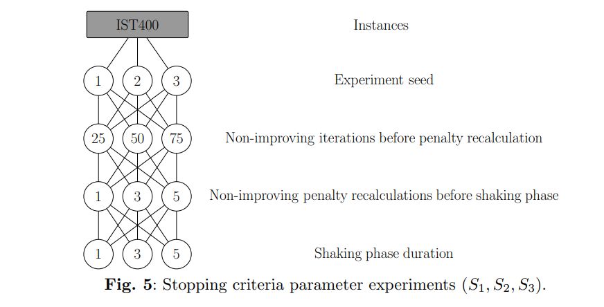
Parameter combinations with a larger S1 allow for greater intensification of a specific search area before inducing the penalty weight recalculation, a diversification mechanism. Changing these penalties changes the trade-off profile between different infeasible solutions. For example, if there has been a time slot that has had a large number of constraint violations for the last iterations, and that number has not improved, the weight for violations on that time slot is increased, and perhaps a new solution can be found with fewer violations on that time slot, even if it has more on another. A shaking phase is introduced if these mechanisms fail to diversify the search to escape a local optimum for S2 recalculations. During this phase, S3 iterations are made without checking if the new solution is better than the previous one. Accordingly, parameter combinations with smaller S1 and S2 are more active in diversifying the search but less precise in identifying local optima. Smaller shaking phases, S3, introduce fewer violations in the new solutions but might not introduce enough change to escape local optima. Each instance and parameter combination is tested with three different seeds to reduce randomness effects. The experiments are summarised in Figure 5.
The average solution time across all 30 instances and for 3 runs of each instance and configuration is presented in Table 2. The five fastest combinations are in bold.
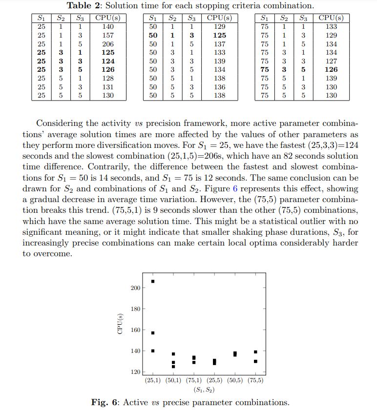
This effect does not mean that more active combinations do not perform very well. Four out of the five fastest combinations can be considered relatively active: (25,3,1), (25,3,3), (25,3,5), and (50,1,3).
5.2 Instance decomposition with fixed curriculum increments
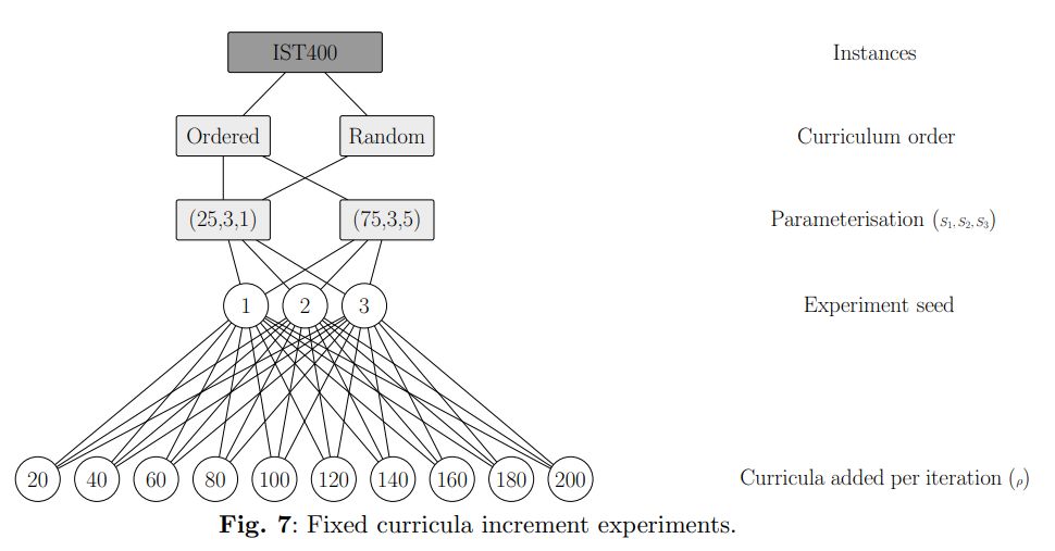
In the previous subsection, the meta-heuristic received the data for all the curricula from the start. In this subsection, we address the experiments regarding fixed curricula increments. The mechanism tested here works as follows: a set of lectures belonging to a fixed number of curricula, ρ, is added to the problem. Then, we find a new feasible solution, s ∗ , considering the current set of lectures, I ′ . When we have a feasible solution, we add the next set of ρ curricula until the complete set is solved. The assignments of each iteration can be changed if necessary in the following iterations.
These experiments test combinations of three factors in the solution times of instances IST400:
– Curriculum order. Randomised curricula increments and ordered increments, following the order from Algorithm 4, which clusters classes based on degrees and years. This means that curricula with more lectures and teachers in common are grouped;
– Parameterisation. Impact of more active (25,3,1) vs more precise (75,3,5) parameter combinations;
– Curricula added per iteration. Number of curricula added in each iteration. The experiments are summarised in Figure 7.
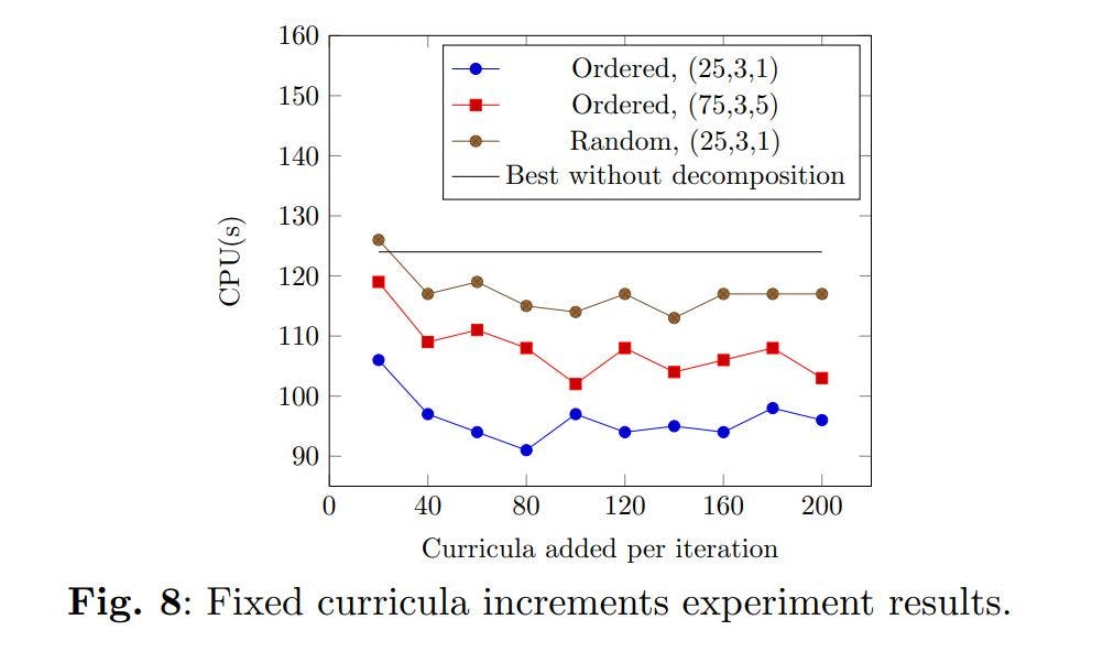
The results show that decomposing and incrementing the problem can reduce solution times to a significant degree. Considering the best curricula added per iteration value, ρ, for each group of experiments: the experiments “Ordered, (25,3,1), ρ = 80” revealed a solution time reduction of 27.2% when compared to the same parameterisation, but without decomposition; the experiments “Ordered, (75,3,5), ρ = 100”, promoted a 20.6% solution time reduction; and the experiments “Random, (25,3,1), ρ = 140”, promoted a 9.6% solution time reduction. These results are presented in Figure 8.
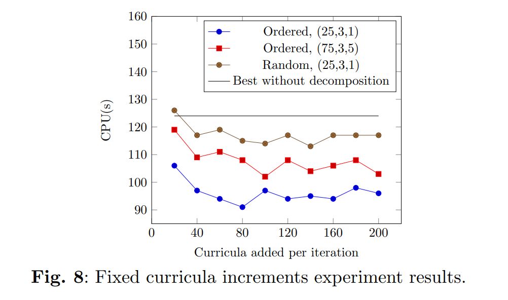
For smaller ρ values, a decrease in this parameter indicates a trend for an exponential increase in solution times. This is an expected behaviour, as if the number of curricula added per iteration is too small, the probability that their timetables might have to be changed in future iterations increases.
The order in which the curricula are added also greatly impacts the efficiency of the methodology, as evidenced by both ordered experiments outperforming the random experiments for every ρ value. The ordering mechanism clusters curricula based on their degrees and years. These results indicate that solving curricula with more classes and professors in common at the same time is beneficial.
To reduce the amount of time the meta-heuristic takes to adjust schedules that will likely need further adjustment in the future, the increments need to be larger. This is especially important when the curricula are not grouped together in the random experiments. Accordingly, these performed better at larger ρ values, 140. Contrarily, the ordered experiments performed better in the 80-100 range. In the ordered experiments, the curricula added in each iteration are less likely to introduce violations based on the assignments of already solved curricula. For example, let us say that three classes from the same year and degree (A, B, C) have to choose two out of three elective courses (1, 2, 3). Class A are the students who choose courses 1 and 2, class B choose 1 and 3, and class C choose 2 and 3. In a random increment, classes A and B might be solved initially, and their entire timetables are built around having lectures from courses 2 and 3 at similar time slots. When class 3 is added later on, these assignments are now infeasible and might be difficult to clear up, as to remove them, some moves which introduce other violations might be necessary. Contrarily, if the increments are made in an ordered manner, this type of situation is less likely to occur.
The parameterisation which is more active in introducing diversification mechanisms (25,3,1), performed better than the parameterisation which intensifies the search more within the same area before diversifying (75,3,5). These combinations are very similar when solving the problems without decomposition, taking, on average, 125s and 126s, respectively. When using decomposition, there are always fewer violations and fewer curricula, professors, and rooms have infeasible schedules during each iteration. This means that local optima are going to be easier to identify. Thus, the extra intensification of a certain area promoted by the combination (75,3,5) is not so beneficial when dealing with a decomposed problem. In this case, active combinations are more efficient, as performing more intensification iterations is less likely to find better solutions.
5.3 Instance decomposition with violations based curriculum increments
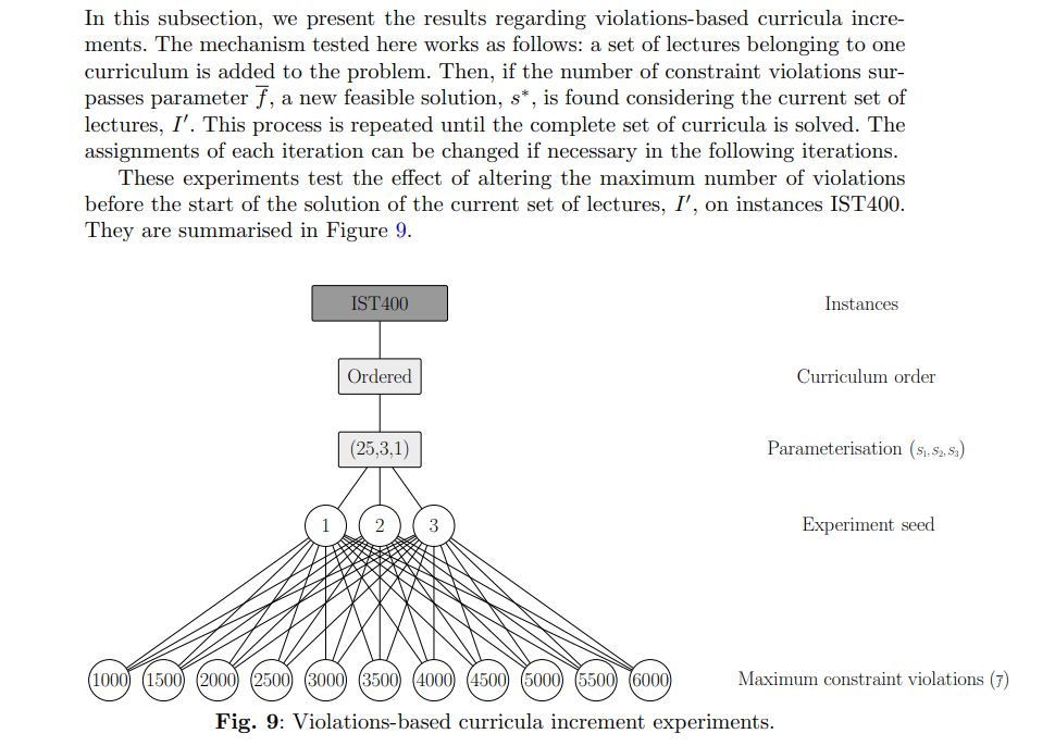
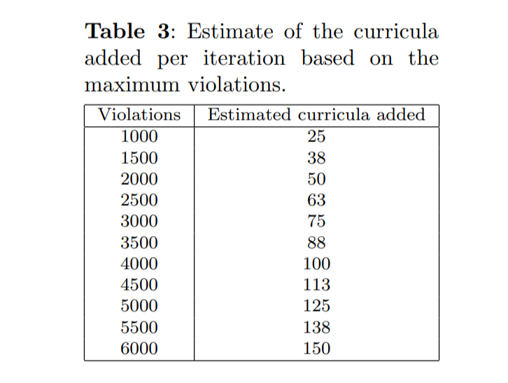
As a reference, 500 violations represent roughly 12.5 curricula. Nonetheless, this value varies quite significantly. Table 3 provides reference values for this estimation.
This mechanism requires the constant generation and assessment of the assignments for each curriculum being added. Comparatively, when doing fixed increments this process is not required. Nonetheless, it presents a trade-off by being more flexible in the number of curricula being added, and doing smaller increments when a feasible solution is expected to be more challenging to find. Figure 10 compares these experiments and the best results of previous experiments.
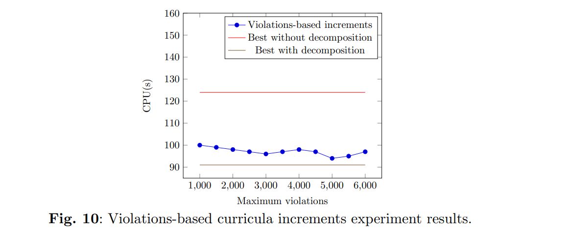
In these experiments, the trade-off of the added flexibility proved insufficient to overcome the added requirements of assessing the violations during the increment phase, and a better average solution time could not be found. Still, the mechanism proved competitive with the previous increment procedure, especially for larger values of estimated curricula added. For the experiments with fewer than 100 estimated curricula added, the violations-based experiments took, on average, between 2 and 5 more seconds than their closest comparison regarding the fixed increment experiments. However, for larger maximum violations limits, they perform very similarly:

5.4 Experiments with larger and real-world instances
In this subsection, we present the results regarding the experiments with the larger subdivisions, IST500 and IST600, which have 500 and 600 curricula, and between 2500 to 2700 and 2800 to 3000 lectures, and with the real-world instance, with 1288 curricula, and 4102 lectures.
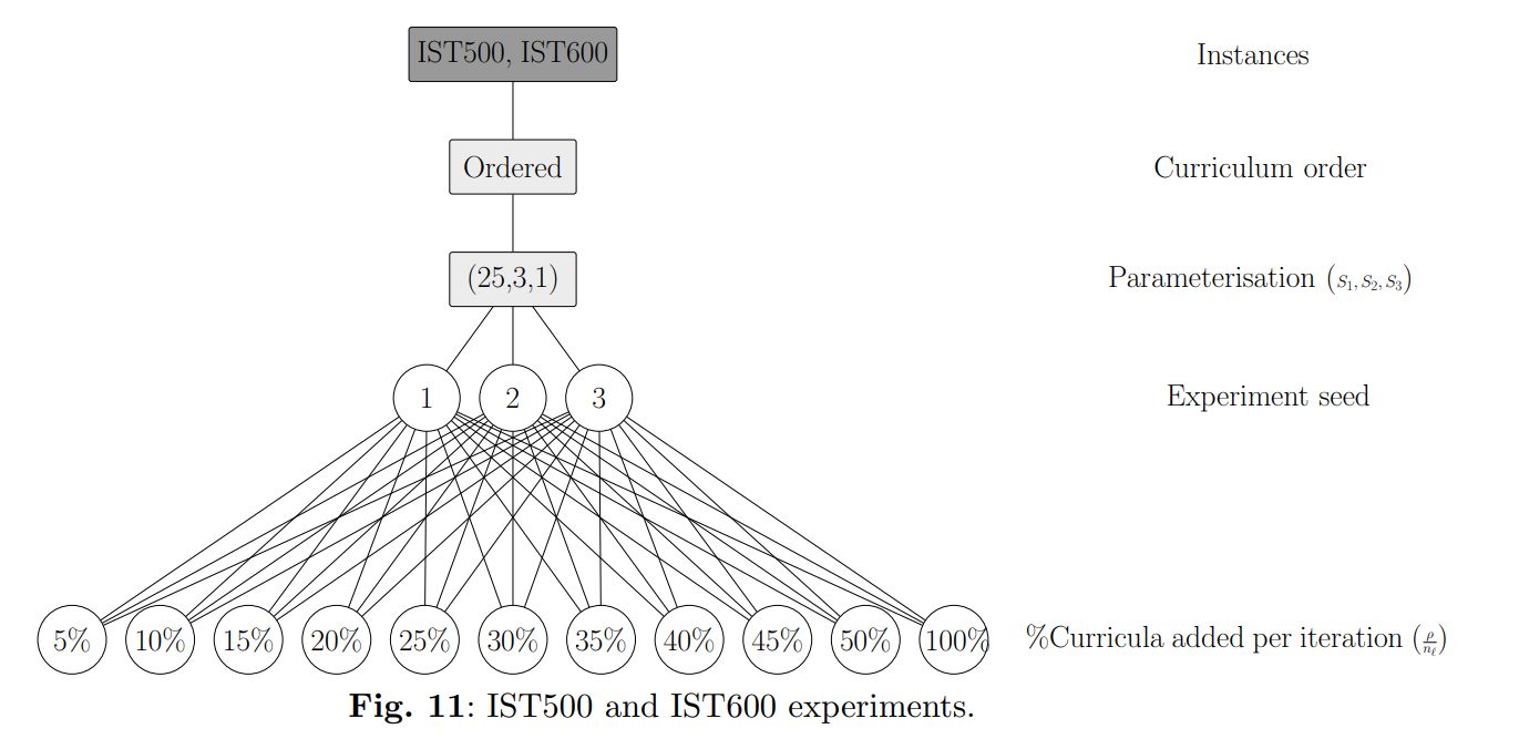
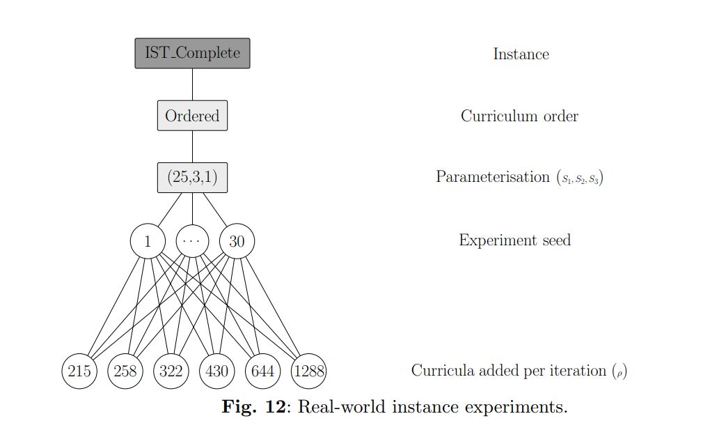
There are some structural differences between the different groups of instances. For example, the IST400 subdivisions kept more than half of the lectures, while including less than a third of the original curricula. This indicates that in the original instance, and in larger subdivisions, the lectures are taught to more curricula on average. Since the subdivisions removed curricula and lectures, and not professors, the professors in the larger instances have considerably more lectures to teach. Finally, the larger subdivisions are increasingly more constrained regarding room availability, and the original instance also presents more room scarcity when compared to instances IST400. The experiments are summarised in Figure 11 for the larger subdivisions and in Figure 12 for the real-world instance. The experiments with 1288 curricula added per iteration are equivalent to solving the problem without decomposition.
Decomposition reduced the solution times by 12.2% for instances IST500, by 8.9% for instances IST600, and by 17.6% for the real-world instance. For the experiments with instances IST400 and IST500, on average, the best curricula added per iteration values represented 20% of the total curricula. However, for instances IST600 and the original instance, the best values are 25% and 50% of the total curricula being added per iteration. The results are presented in Figure 13 for instances IST500, in Figure 14 for instances IST600, and in Figure 15 for the real-world instance.
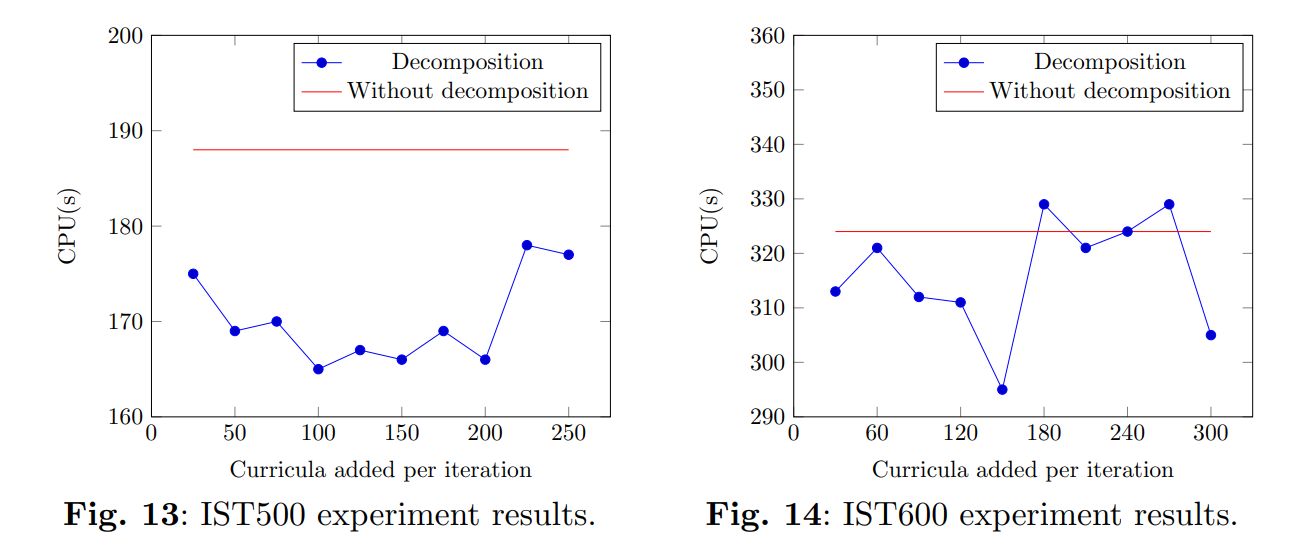
The structural differences between the instances can explain this discrepancy in results. If a lecture is shared between multiple curricula, it is more likely that introducing curricula that include said lecture will create constraint violations in the decomposed problem. Likewise, if the professors have more lectures to teach, adding more lectures to the problem has a greater probability of making their timetables infeasible. In practice, this translates into larger increments being more efficient for the more complete instances, as they have more interdependencies between curricula. Finally, in instances where there are fewer available rooms per lecture, the introduction of new lectures may violate the room availability constraints. All of these concerns translate into more changes being required to solve constraint violations when incrementing the problem, as each set of curricula is less contained in itself, i.e., there is more interaction between different curricula, reducing the relative effectiveness of the decomposition strategy.
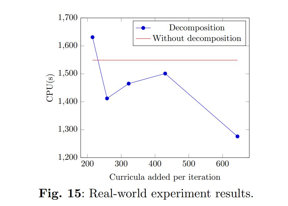
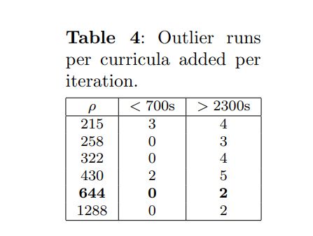
When solving a decomposed instance there is a trade-off between the amount of time required to adjust timetables which become infeasible after an increment, which is reduced by doing larger increments, and the simplicity of each iteration, which is increased by doing smaller increments. This simplicity promotes the possibility of using faster diversification rates and facilitates the identification of the time slots with the most violations and the most challenging constraint violation groups. In Table 4, both the number of runs per ρ value that took less than 700 seconds and more than 2300 seconds for the real-world instance is presented. In general, smaller increments have an increased likelihood of producing both very fast and very slow runs. We speculate that even for these parameterisations, sometimes the generated assignments do not require a significant amount of changes. In these cases, the added simplicity can promote very efficient runs. Nonetheless, the opposite can happen, and the generated assignments require several corrections, resulting in slower solution times. These results suggest that further improvements can be made to the methodology if tighter curricula clusters can be created, enabling smaller increments without requiring as much ineffective work as they would have fewer interactions amongst each other.
5.5 Competition instances
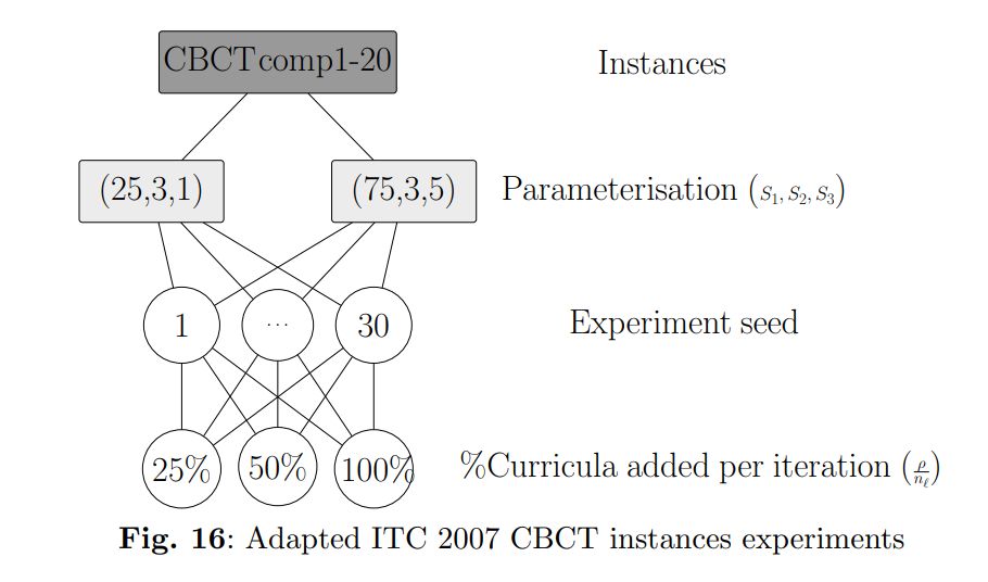
In this subsection, we present the results regarding the experiments with the adapted benchmark instances from the CBCT competition track of ITC 2007. Maximum consecutive workload, precedence, and different day lecture constraints were added to the original instances, and unavailable slots were not regarded. Each of the twenty instances was run with 30 different seeds for parameterisations (25,3,1) and (75,3,5), with 25%, 50%, and 100% of their curricula added per iteration. The experiments are summarised in Figure 16.
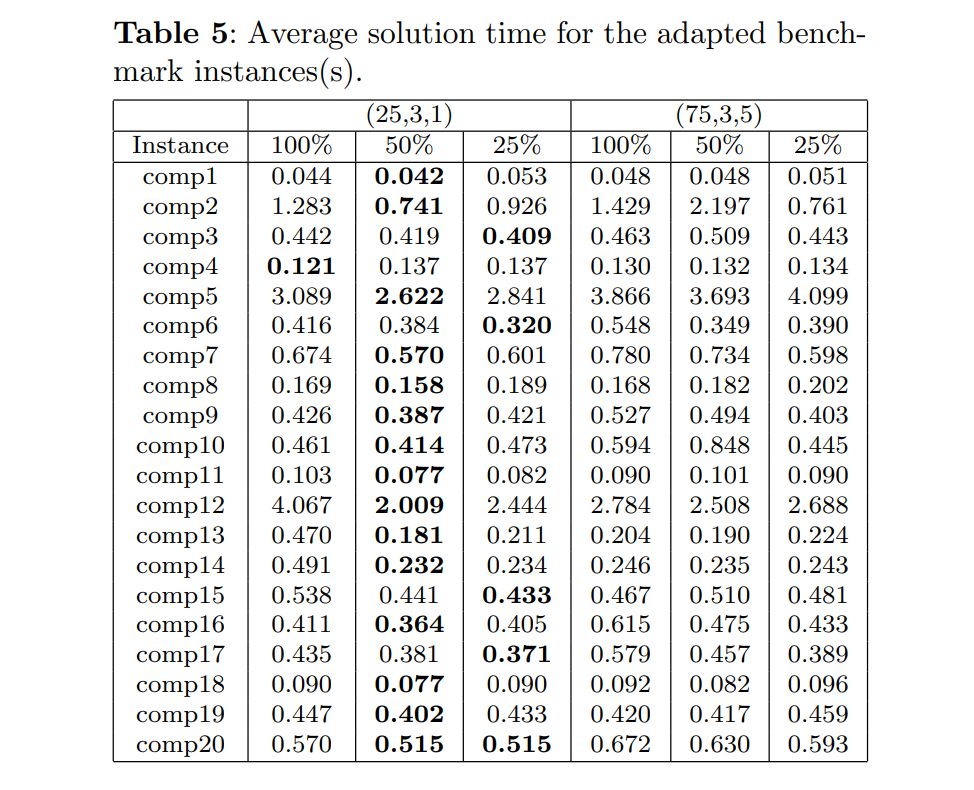
The parameterisation (25,3,1) with 50% of curricula being added per iteration was the fastest configuration for 15 out of the 20 tested instances. Since these instances are not very complex, this parameterisation, which diversifies the search faster, performed better. Moreover, making divisions smaller than 50% of the curricula was also ineffective, as the number of curricula does not justify such small increments. The results are presented in Table 5.
This paper is available on arxiv under CC 4.0 license.

