Authors:
(1) Jo˜ao Almeida, CEGIST, Instituto Superior T´ecnico, Universidade de Lisboa Portugal;
(2) Jos´e Rui Figueira, CEGIST, Instituto Superior T´ecnico, Universidade de Lisboa Portugal;
(3) Alexandre P. Francisco, INESC-ID, Instituto Superior T´ecnico, Universidade de Lisboa Portugal;
(4) Daniel Santos, CEGIST, Instituto Superior T´ecnico, Universidade de Lisboa Portugal.
4 Algorithmic framework
In this section, we explain the algorithmic framework of our meta-heuristic. In Subsection 4.1, we give a general overview. In Subsection 4.2, we introduce the instance decomposition and increment procedure. In Subsection 4.3, we present the heuristic for generating the initial timetables. In Subsection 4.4, we address the guided local search component. In Subsection 4.5, we address the adaptive large neighbourhood component. In Subsection 4.6, we address the variable neighbourhood search component.
4.1 Overview
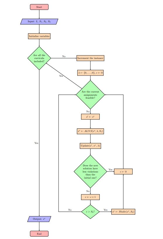
Our hybrid meta-heuristic uses mechanisms from adaptive large neighbourhood search (ALNS), guided local search (GLS), and variable neighbourhood search (VNS). Its generic representation is presented in Figure 1. Its inputs are the full set of curricula, L, and three stopping criteria, S1, S2, and S3. Additional parameters are also necessary for its functions and procedures, which are addressed in the following subsections. Its output is a feasible schedule, s∗ .
Instead of solving the entire instance from the start, we decompose it by curricula and increment it iteratively until the set of curricula being solved, L′ , is equal to the entire set of curricula, L. The decomposition mechanism functions in the following way: a set of lectures belonging to a set of curricula is added to the problem. Then, we find a new feasible solution, s∗ , considering the current set of lectures, I′. When we have a feasible solution, we add the next set of curricula. Let us note that the assignments of each iteration can be changed if necessary in the following iterations.
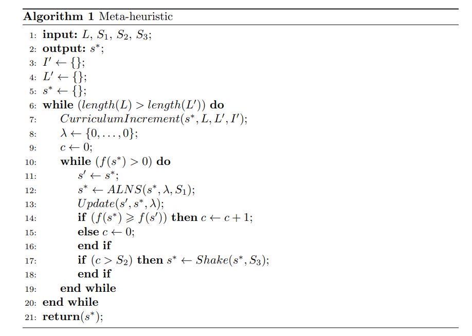
Our objective function, f(s ∗ ), represents the number of hard constraint violations in the current solution. Thus, the neighbourhoods are searched to find if there is a neighbour with fewer violations. The neighbourhood structures are explained in detail in Subsection 4.5. However, instead of using a regular objective function in this search, we introduce mechanisms for penalising certain features in the solution, which are useful for escaping local optima. Accordingly, after a certain number of iterations, the feature penalty vector, λ, is updated. The features and the update procedure are explained in detail in Subsection 4.4. However, sometimes this penalty is not enough to escape some local optima. To avoid those, we include a shaking phase, which occurs after a certain number of penalty recalculations without improvements. The number of local searches before updating the penalty vector is the stopping criterion S1. The number of penalty weight recalculations which is attempted before inducing a shaking phase is the stopping criterion S2. The duration of the shaking phase is the stopping criterion S3. The pseudo-code for this meta-heuristic is presented in Algorithm 1.
4.2 Instance decomposition and increment
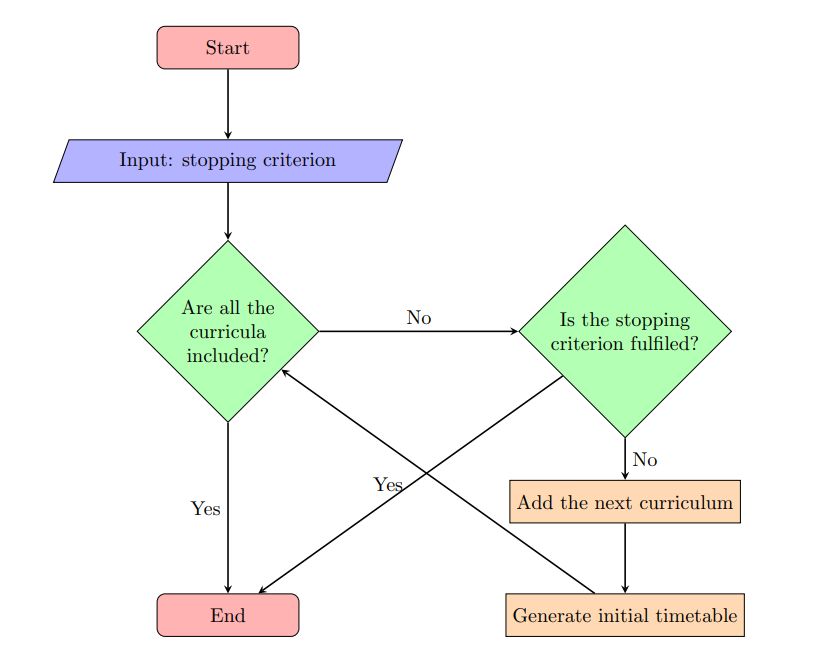
The procedure to increment the instance is straightforward. Curricula are added to the instance until a specific stopping criterion is met, or the entire set of curricula is included.
We explore two different stopping criteria. One receives as input a fixed number of curricula to be added in each iteration, ρ. The other adds curricula until a certain number of hard constraint violations, f, is reached. Their respective pseudo-code algorithms are given in the Appendix. Algorithm 8 presents the fixed increments procedure and Algorithm 9 the violations-based increment procedure.
Whenever a new curriculum, ℓ ′′, is added, its lectures, i ∈ aℓ ′′ , must be scheduled and added to the current solution, s∗ . The function which returns the schedule for each new curriculum is presented in the following subsection.
Figure 2 provides a diagram of the procedure.
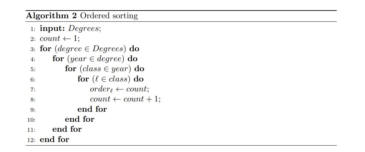
We test two different sorting algorithms for deciding the order in which the curricula are added. The random sorting procedure chooses a random curriculum. The ordering procedure picks a degree, then, by ascending order of year, picks a class, and then adds the first and second trimesters, each corresponding to a different curriculum, ℓ, or timetable. This procedure is presented in Algorithm 2.
4.3 Initial solutions
4.4 Guided local search
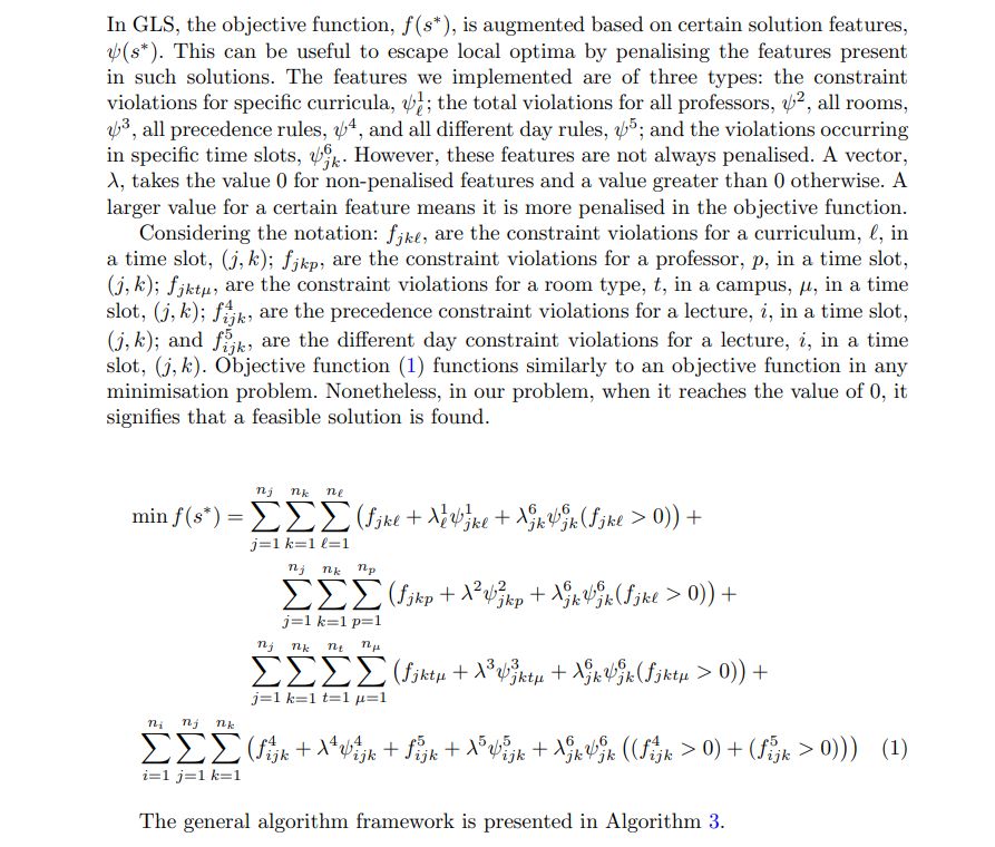
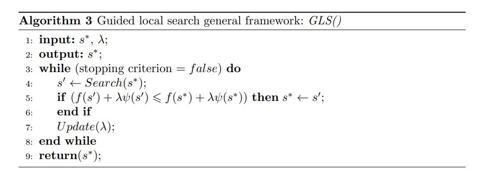
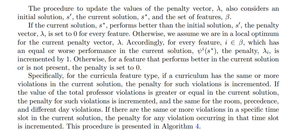
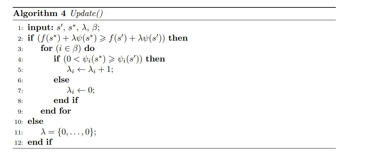
Considering each type of constraint violation as an objective, this methodology can be analysed as a multi-objective search technique. Effectively, what is happening is that out of the objective functions being regarded, the most challenging to improve are identified. Then, their weights, λi , are updated to help the search move towards non-dominated solutions that improve these objectives’ performance, even if the total sum of the effective violations increases.
4.5 Adaptive large neighbourhood search
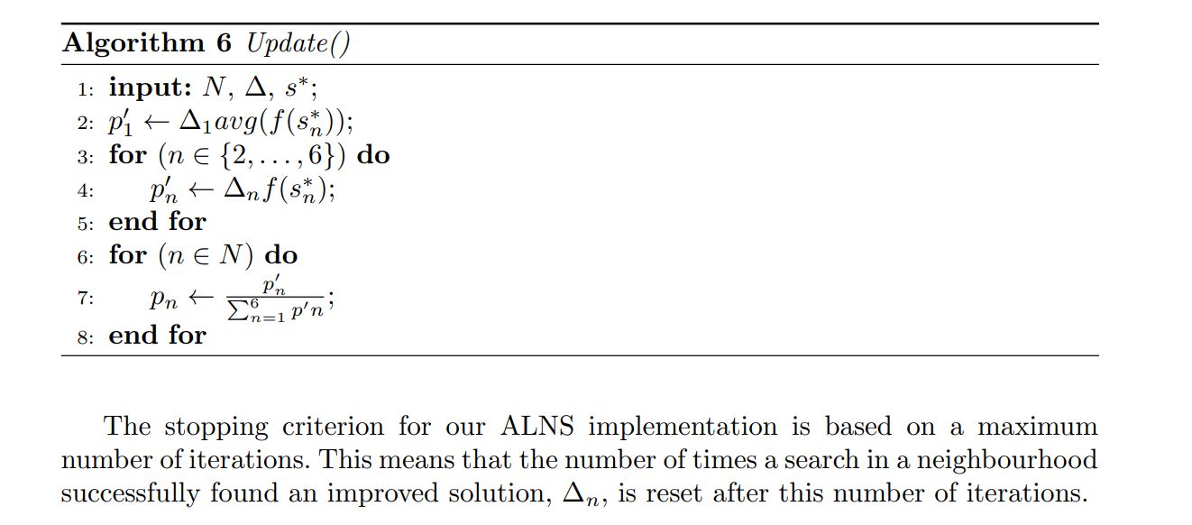
In ALNS, the local search is based on different neighbourhood structures. In each iteration, a neighbourhood structure, n, is selected based on a probability vector, p, and a local search is conducted. If a better solution is found, it replaces the bestknown solution. Let us note that we use an augmented objective function adapted from GLS procedures, f ′ (s). Then, based on the current solution characteristics and the previous successes of searches in each neighbourhood, the probability vector, p, is updated. The general algorithm framework is presented in Algorithm 5.
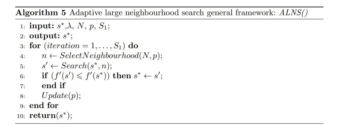
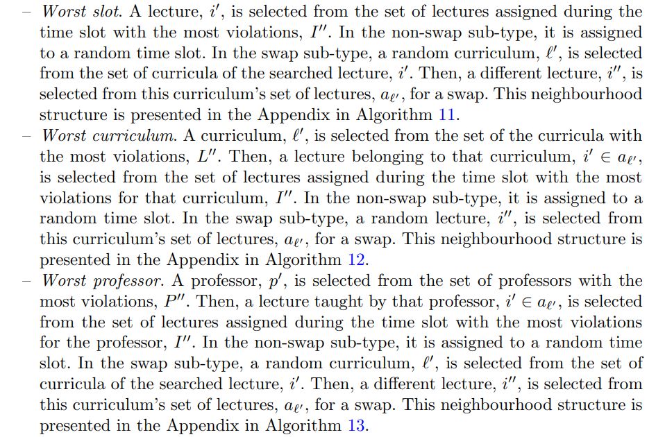
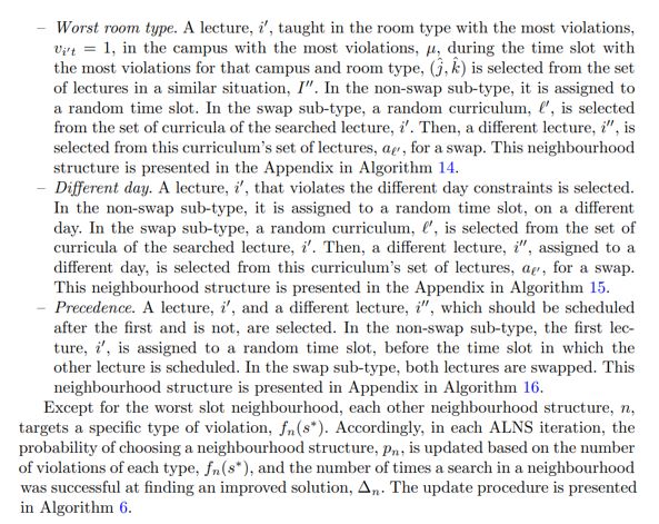
To implement ALNS, it is necessary to define the set of neighbourhood structures, N, the procedure for updating the probability vector, p, and the stopping criterion. We established six main neighbourhood structures, which we named: worst slot, worst curriculum, worst professor, worst room type, different day, and precedence neighbourhoods. Moreover, each of them has two sub-types, named swap and non-swap. In each neighbourhood, a lecture is selected, and then, in the swap sub-type, its time slot is swapped with another lecture, and in the non-swap sub-type, it is randomly assigned to another time slot.
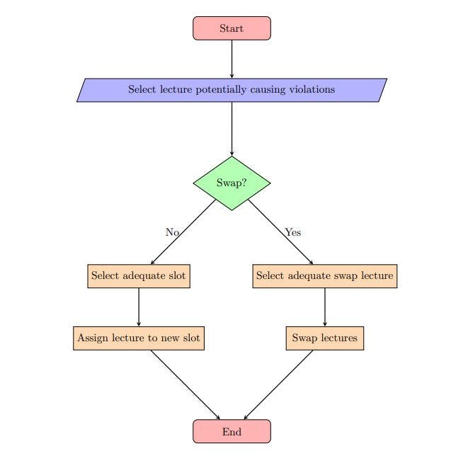
The neighbourhoods follow a general framework that can be applied to each type of constraint violation. The first step is randomly selecting a lecture potentially causing violations. Then, either an adequate new time slot or an adequate swap lecture is randomly assigned. This adequacy is assessed based on the type of violation being caused. This general framework is presented in Figure 4.

Specifically, each neighbourhood structure operates in the following manner:
4.6 Variable neighbourhood search
In VNS, whenever local optima are identified, a shaking phase is used to move to different areas of the solution space. In our meta-heuristic, such a shaking phase is conducted if no improvement moves are found after a certain number of feature penalty updates are made. This shaking phase functions similarly to the ALNS algorithm, but every move is accepted instead of only those which introduce improvements. This phase is stopped after a number of iterations, S3. It is presented in Algorithm 7.

This paper is available on arxiv under CC 4.0 license.

