Authors:
(1) Renan F. F. da Silva, Institute of Computing, University of Campinas;
(2) Yulle G. F. Borges, Institute of Computing, University of Campinas;
(3) Rafael C. S. Schouery, Institute of Computing, University of Campinas.
8 Computational Results
Next, we present the instances used in our experiments [1] . Sequentially, we show some results comparing our algorithms in two-stage. We compare our initial heuristics using a performance profile and statistic tests in the first stage. In the second stage, we make a statistical comparison between the VNS and the MH.

8.1 Instances
The instances used in experiments have four classes.
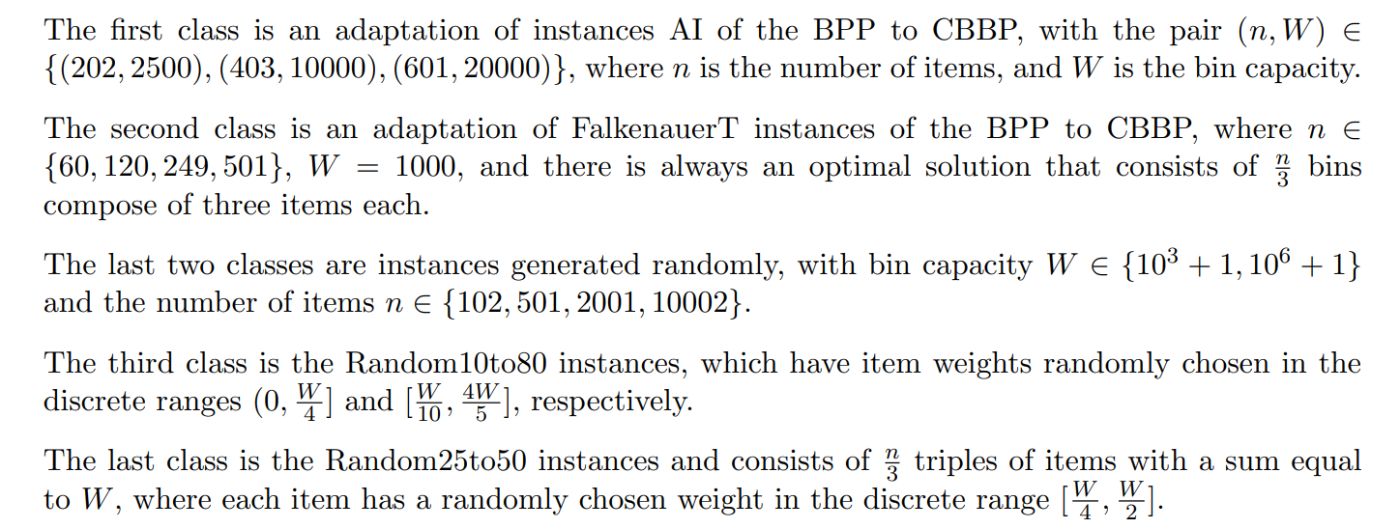
The BPP instances AI and FalkenauerT are available in the BPP Lib created by Delorme et al [15], and their optimal solutions are known. In the BPP, AI instances are very hard instances to find an optimal solution, but they are easy to find a solution with an extra bin. The instances FalkenauerT and Random25to50 are similar, but we create the Random25to50 because FalkenauerT does not have instances with a large number of items or a large bin capacity.

8.2 Comparison between Initial Heuristics
Next, we compare our initial heuristics using a performance profile and statistic tests.
8.2.1 Performance Profile
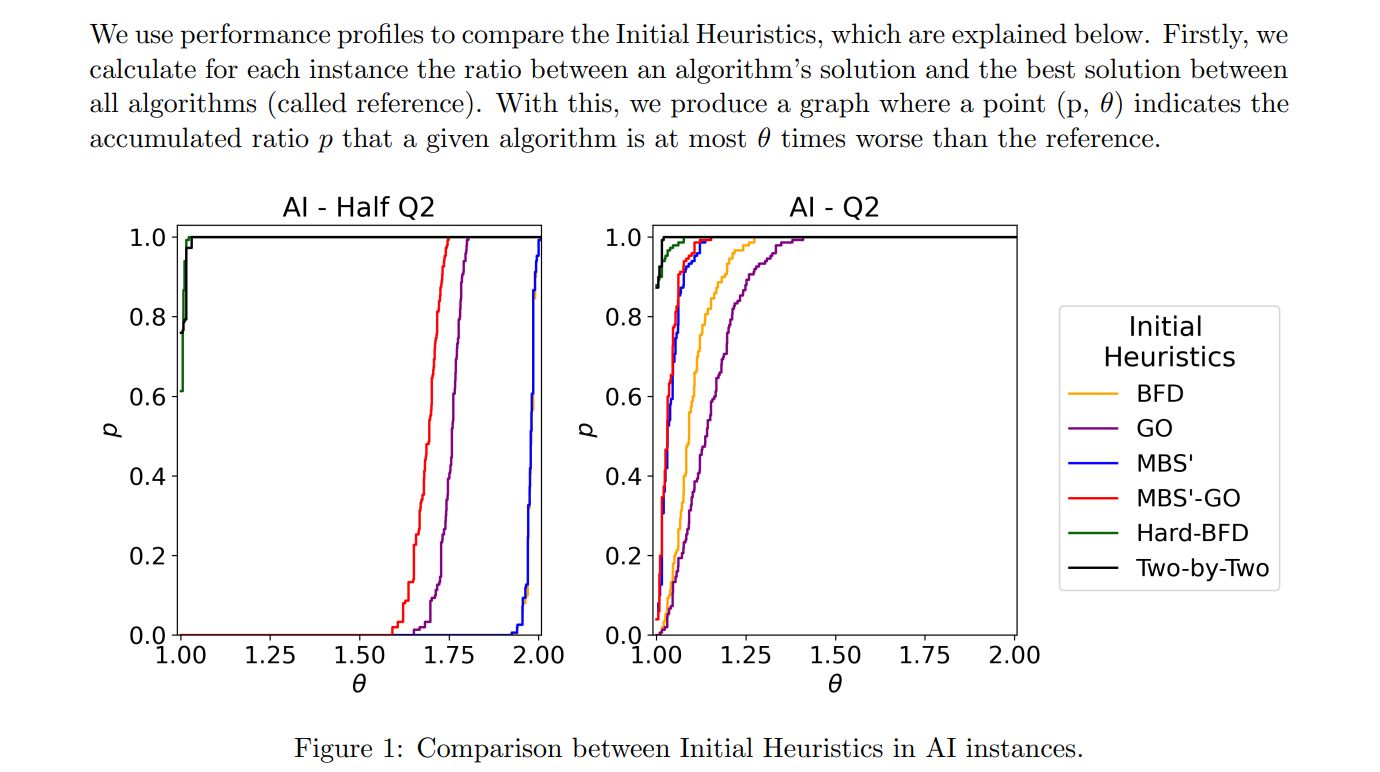
In Figure 1, we have the performance profile for the combinations of AI instances with the coloring Q2 and Half Q2. As we can see, the heuristic Two-by-Two is the best, being up to two times better than the BFD in some instances in coloring Half Q2. The graph for the other coloring is similar to Q2, but the difference decreases as we increase the number of colors. This behavior also happens in other instances, so we omit the graphs for these coloring.
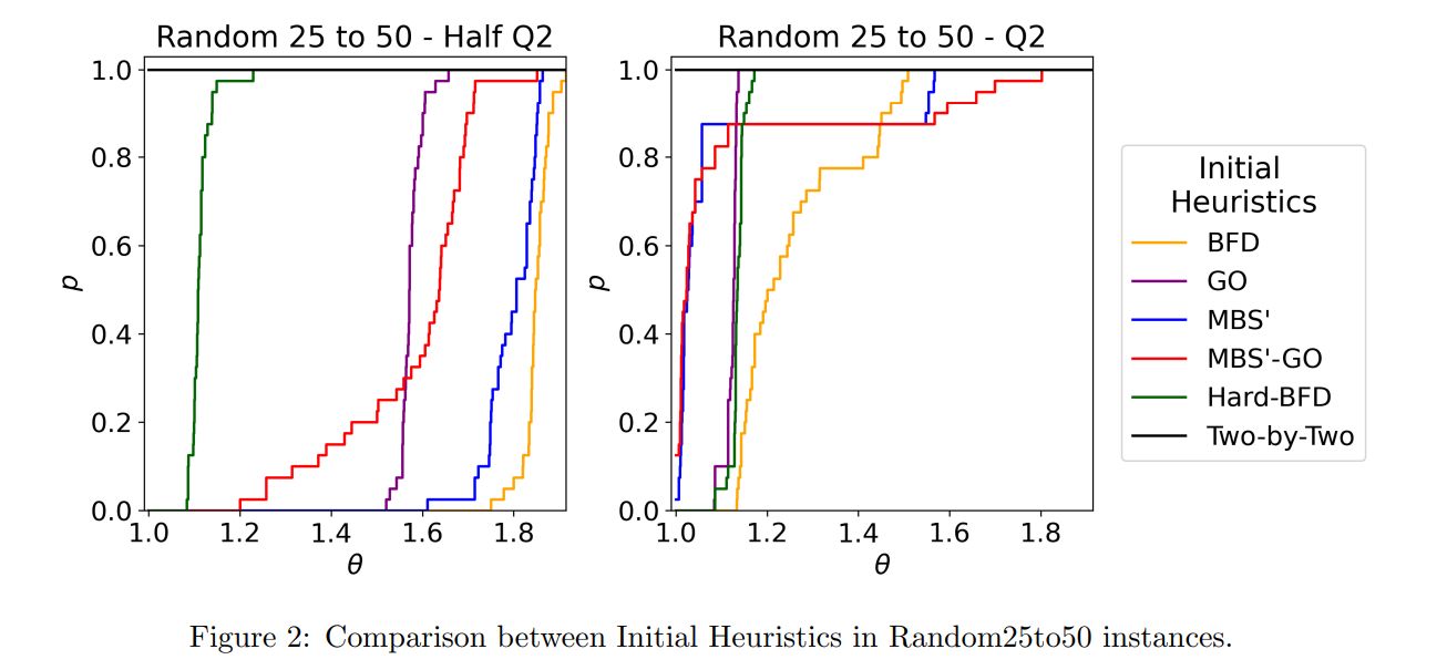
Figure 2 presents the results for Random25to50 instances with coloring Q2 and Half Q2. Again, the heuristic Two-by-Two is the best one. This time, it has a reasonable superiority to Hard-BFD, which use at least 10% more bins. See that the two MBS’ versions are curiously better than the Hard-BFD in 90% of the instances with Q2. The results for the FalkenauerT instances are similar to Random25to50.
Next, in Figure 3, we have the performance profile for Random10to80 with coloring Q2 and Q5. Observe that with the coloring Q2, we do not have a clear dominance between the heuristics Twoby-Two and Hard-BFD.
Finally, note that the good-ordering often improves the solution quality, but exceptions exist. For example, the Good Ordering heuristic is worse than the BFD heuristic in AI instances with Q2.
8.2.2 Statistic Tests

The comparison we made is based on non-parametric analysis, as was made by Demˇsar [16]. As we can compare multiple strategies on a set of different instances, we use the adaptation of the Friedman test (Friedman [20]) made by Iman and Davenport [24], rejecting the null hypothesis when the value of the test is greater than the critical one according to the F-distribution. In such a case, we proceed with a post hoc analysis using the Nemenyi test (Nemenyi [29]) to identify the group of statistically equivalent strategies. This situation is identified when the average ranks of two samples differ at most by a given critical difference (CD).
Our test has k = 6 algorithms and N = 1200 instances. For these parameters, the critical value of the F-distribution is 2.22. Next, we can compute the test value FF to the Iman-Davenport, where our data has FF = 484.02. As FF is greater than the critical value, the null hypothesis H0 was rejected, and we accepted the alternative hypothesis H1. Therefore, we can apply the Nemenyi test to determine which heuristics have statistical differences.
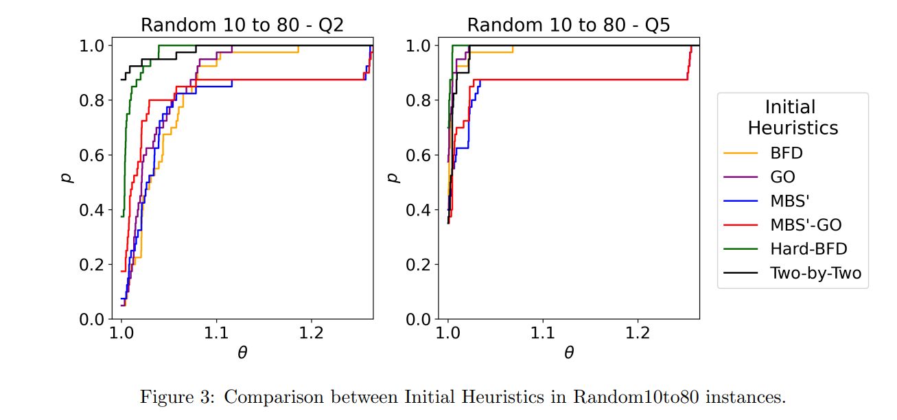
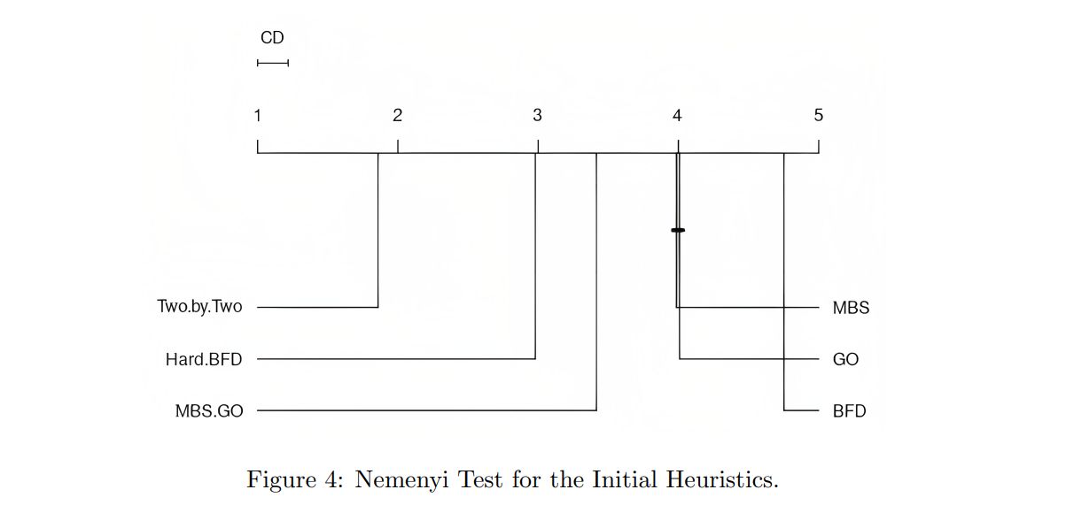
Figure 4 presents a graph illustrating the Nemenyi test. For our data, we have the critical difference CD = 0.22. The heuristic average ranks are classified from left to right, where the better heuristic is the most on the left. If two heuristics have average ranks with a difference less than the CD, then they are connected by a horizontal line, which means that we did not find a statistical difference between them. As we can see in the figure, the Two-by-Two is the best heuristic. Note that the “good-ordering” is beneficial in the general case since MBS’-GO and GO heuristics perform better than their original versions MBS’ and BFD. Finally, we do not find a statistical difference between MBS’ and GO heuristics.
8.3 Comparison between VNS and MH
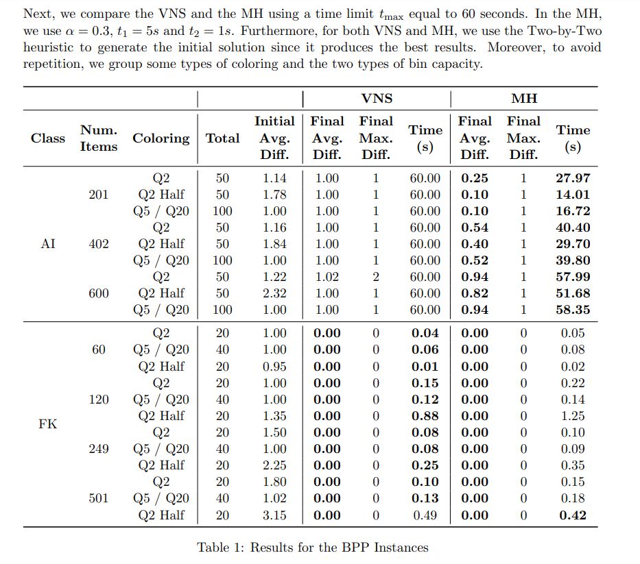
In the Tables 1 and 2, the columns “Initial Avg. Diff.” e “Final Avg. Diff.” indicate the average differences between the lower bound L1 and the initial and final solution values, respectively. The column “Final Max. Diff.” indicate the maximum difference of a final solution about lower bound L1. Moreover, the column “Time” gives the average time in seconds. Finally, we highlight in bold
the best “Final Avg. Diff.” of each line.
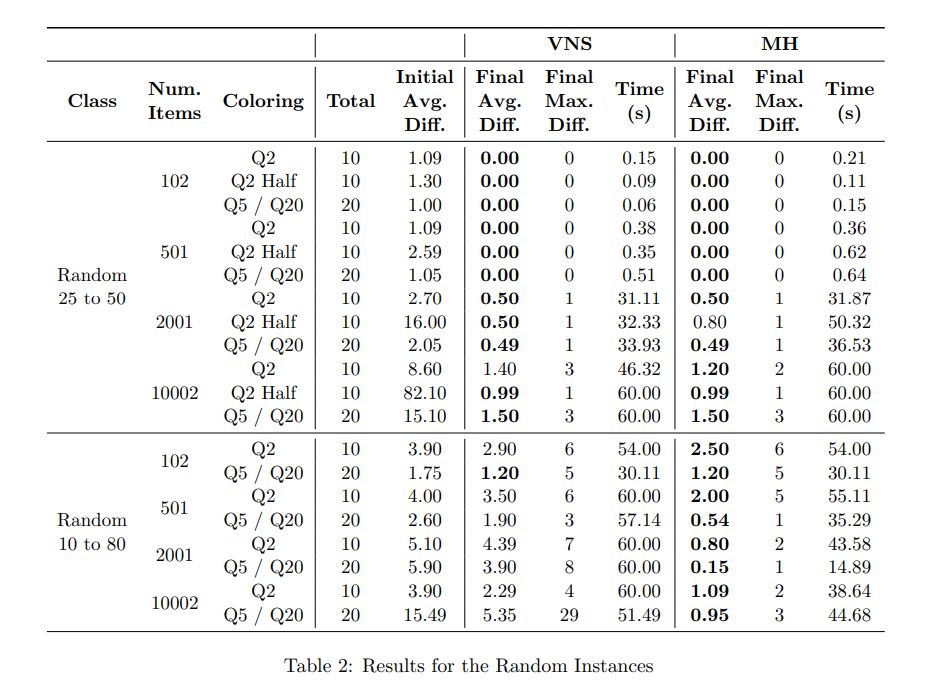
As we can see, our approaches obtained good results since they optimally solve all Random25to50 instances with 102 and 501 items and find solutions with at most one extra bin than the optimal solution with 2001 items. Moreover, we can emphasize this class with 10002 items and coloring Half Q2, where the average initial difference is 82.1 bins, and our approaches decrease this difference to at most 1 bin.
Besides, our approaches also solve all FalkenauerT (FK) instances. Note that there is no clear relation between difficulty and the number of items since instances with 120 items and Half Q2 are the most costly in execution time.
Moreover, see that the coloring Half Q2 has the greater initial average difference in all instance classes. However, it is not necessarily reflected in more hard instances since in some cases, the final maximum difference is slightly smaller in this coloring.
Finally, our MH is superior to VNS since the MH optimally solves 124, 70, and 9 of the 150 AI instances with 202, 403, and 601 items, respectively, while the VNS does not solve any of them. Moreover, in some cases, the average final difference in Random10to80 instances is several times smaller in MH than in VNS. Note that the average difference in the final solutions is less than 3 in the MH. This difference is significantly greater in Random10to80 instances, where L1 is probably not a tight lower bound.
[1] All instances and source codes are available at https://gitlab.com/renanfernandofranco/
fast-neighborhood-search-heuristics-for-the-colorful-bin-packing-problem.
This paper is available on arxiv under CC 4.0 license.

